


Cara menggunakan VLOOKUP di Excel - tutorial sederhana (bagian I)
Excel function tutorials Fungsi excel tutorial

If you use Excel much at your job, sooner or later, you're bound to need to look up values in a table. Jika Anda menggunakan Excel banyak di pekerjaan Anda, cepat atau lambat, anda pasti akan perlu untuk melihat nilai-nilai di atas meja. One of the most useful functions in Excel, called vlookup , does exactly that. Salah satu fungsi yang paling berguna dalam Excel, yang disebut vlookup, yang tidak tepat. The “V” in vlookup stands for “vertical” and “lookup” is pretty self explanatory. The "V" di vlookup adalah singkatan "vertikal" dan "lookup" is pretty self explanatory. This function allows you to look up values in a table that are listed in column format (how most tables are laid out), given another value (let's call this the “key”). Fungsi ini memungkinkan Anda untuk mencari nilai-nilai dalam tabel yang tercantum di kolom Format (cara paling meja laid out), yang lain diberi nilai (mari kita menyebutnya dengan "kunci"). Excel also has a sister function called hlookup (h = horizontal) that can be used to look up values in rows. Excel juga memiliki fungsi saudara perempuan bernama hlookup (h = horisontal) yang dapat digunakan untuk mencari nilai dalam baris.
Sadly, as most companies seem to rely on Excel as a poor-man's database of sorts (a totally unscalable solution and prone to errors with every revision, but don't get me started), once you know vlookup, it's likely to become one of your most often used Excel functions. Sayangnya, seperti kebanyakan perusahaan tampaknya mengandalkan Excel sebagai orang miskin-jenis database (a totally unscalable solusi dan rentan terhadap kesalahan dengan setiap revisi, tetapi tidak mendapatkan saya mulai), setelah Anda tahu vlookup, kemungkinan untuk menjadi satu Anda paling sering digunakan fungsi Excel.
So, let's get started with a very simple example of what vlookup is all about. Jadi, mari kita mulai dengan contoh yang sangat sederhana dari apa vlookup adalah semua tentang. Suppose you had the following table: Misalnya anda mempunyai tabel berikut:
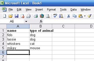
Given a list of names in another part of the table (in this case, column H), you want to figure out what kind of animal it is: Diberikan daftar nama di bagian lain dari tabel (dalam hal ini, kolom H), Anda ingin mengetahui jenis hewan itu adalah:

Vlookup's format looks like the following: Vlookup dari format seperti berikut ini:
Let's look at each of these parts a bit closer. Mari kita melihat tiap-tiap bagian sedikit lebih dekat.
The first thing that goes into the vlookup function is the thing you know (or are given) and that will be used to lookup other values. Hal pertama yang masuk ke dalam fungsi vlookup adalah hal yang Anda tahu (atau diberi) dan yang akan digunakan untuk mencari nilai-nilai lain. In this case, you have the names of the animals, so these are the things we know. Dalam hal ini, Anda memiliki nama-nama hewan, jadi ini adalah sesuatu yang kita tahu. In our example, they reside in column H, from cells H2 through H5. Dalam contoh kita, mereka berada dalam kolom H, dari sel H2 melalui H5. If we wanted to put the type of animal next to the name of the animal in column I (so I2 would correspond to the name of the animal in H2), we would insert the vlookup function there: Jika kita ingin menempatkan jenis hewan di samping nama dari binatang di kolom saya (I2 sehingga akan sesuai dengan nama hewan di H2), kami akan memasukkan fungsi vlookup sana:

and put H2 as the first thing in our vlookup function: H2 dan diletakkan sebagai hal pertama di vlookup fungsi:

Next, we need to know the location of the table where our values reside. Selanjutnya, kita perlu mengetahui lokasi dari tabel nilai-nilai di mana kami berada. These happen to be from cells A1 through B5 in this example, which we would highlight with our mouse to insert into the vlookup function. Ini akan terjadi dari sel A1 melalui B5 dalam contoh ini, yang kita sorot dengan mouse untuk memasukkan ke dalam fungsi vlookup. It's very important that you include all the cells in the table. Ini sangat penting bahwa Anda memasukkan semua sel dalam tabel.
Highlight the table with your mouse: Sorot tabel dengan mouse:

At the same time, the vlookup function automatically puts in the cells you've highlighted: Pada saat yang sama, maka secara otomatis akan menempatkan vlookup dalam sel Anda disorot:

Next, we need the column number where the values are located. Selanjutnya, kita perlu kolom nomor dimana nilai berada. Always start with the first column (column A in this case) as #1 and count out to the right. Selalu mulai dengan kolom pertama (kolom A dalam hal ini) sebagai # 1 dan mengeluarkan ke kanan. In this example, the type of animal listed is in column 2, so that's what we would need to insert in the vlookup function. Dalam contoh ini, jenis hewan yang tercantum dalam kolom 2, sehingga dari apa yang kita akan perlu untuk memasukkan dalam fungsi vlookup. Note that to use vlookup, your keys always have to be to the left of your values. Perlu diketahui bahwa untuk menggunakan vlookup, kunci selalu harus di sebelah kiri Anda nilai. (We'll cover more of this in part II of the tutorial at a later date.) (Kami akan mencakup lebih dari ini di bagian II dari tutorial di kemudian hari.)

Finally, the last attribute that vlookup takes is either “true” or “false”. Akhirnya, yang terakhir atribut vlookup berlangsung baik adalah "true" atau "palsu". I happen to always use “false”, and what this does is force vlookup to return the first exact value it finds. Saya selalu terjadi menggunakan "palsu", dan apa ini tidak akan memaksa untuk kembali vlookup pertama ia menemukan nilai tepat. If that value isn't found, then vlookup conks out and returns “#N/A”. Jika nilai yang tidak ditemukan, maka vlookup conks dan kembali "# N / A". Though we won't use it in this example, if you select “true”, then rather than always looking for the exact value, vlookup will return the exact value if it exists, or the closest one to it that doesn't exceed the key. Meskipun kami tidak akan digunakan dalam contoh ini, jika Anda memilih "benar", maka daripada selalu mencari nilai yang tepat, vlookup akan mengembalikan nilai yang tepat jika ada, atau yang paling dekat ke salah satu yang tidak melebihi kunci. (If you use “true”, you will need to sort your data in ascending order before using vlookup.) (Jika anda menggunakan "benar", Anda perlu menyusun data Anda naik di urutan sebelum menggunakan vlookup.)

Still with me? Masih dengan saya? Again, this is what we would actually put in cells I2 if the names of the animals we have are located in cells H2 through H5: Sekali lagi, ini adalah apa yang kita benar-benar akan dimasukkan ke dalam sel I2 jika nama-nama hewan kami telah berada di sel H2 melalui H5:
Once we close off the parenthesis and hit “Enter”, vlookup automatically calculates: Setelah kami tutup kurung mematikan dan tekan "Enter", vlookup otomatis menghitung:

And so on. Dan sebagainya. We would continue down each cell in column I that we needed. Kami akan terus turun setiap sel dalam kolom saya bahwa kami diperlukan. One thing to note is to make sure that the location of your keys and values is always selected correctly. Satu hal yang perlu diperhatikan adalah untuk memastikan bahwa lokasi kunci dan nilai-nilai yang selalu dipilih dengan benar. Oftentimes, as you copy-and-paste formulas all around Excel, the location of the data will also move around relative to the cell. Sering kali, karena anda meng-copy-paste seluruh rumus Excel, lokasi data juga akan berpindah ke sel relatif. The easiest way to prevent this is to “lock” the range of the location; in this case, we would do so by using “$A$1:$B$1″ instead of “A1:B5″. Cara termudah untuk mencegah hal ini adalah "kunci" di berbagai lokasi, dalam hal ini, kami akan melakukannya dengan menggunakan "$ A $ 1: $ B $ 1" bukan "A1: B5". This way, as we move down column I, say, to cell I2, A1:B5 doesn't become A2:B6 but stays with the original range of data. Dengan cara ini, karena kami bergerak bawah kolom I, mengatakan, ke sel I2, A1: B5 tidak menjadi A2: B6 tetapi tetap asli dengan berbagai data. This way, we can just copy what's in cell I2 down the rest of the cells (from I3 through I5): Dengan cara ini, kami hanya dapat menyalin apa dalam sel I2 bawah bagian sel (dari I3 melalui I5):

Finally, here's our result, after making the “$” changes and copying and pasting the formula down the rest of the column: Akhirnya, kami di sini dari hasilnya, setelah membuat "$" perubahan dan mengcopy paste rumus bawah sisa kolom:

This has been a really simple example of vlookup, and I'll cover a bit more in part II with another example, still simple, but with slightly more data. Ini telah menjadi contoh yang sangat sederhana vlookup, dan saya akan membahas sedikit lebih dalam bagian II dengan contoh lain, masih sederhana, tetapi dengan sedikit lebih banyak data.
Although in practice, vlookup is usually used between Excel sheets and workbooks, once you understand this example (which has been done within a single sheet), using vlookup outside the same sheet shouldn't be much harder. Meskipun dalam praktiknya, vlookup biasanya digunakan antara lembar dan workbook Excel, setelah Anda memahami ini contoh (yang telah dilakukan dalam satu lembar), menggunakan vlookup luar lembaran yang sama seharusnya tidak akan jauh lebih keras. Look for part II soon! Mencari bagian II segera!


0 komentar:
Posting Komentar